The original data of Jin et al 2020 can be downloaded from the Broad single cell portal (https://singlecell.broadinstitute.org/single_cell/study/SCP1184). Here, we just use a subset of the data to demonstrate the workflow of the analysis.

library(Seurat)

## Loading required package: SeuratObject

## Loading required package: sp

## 'SeuratObject' was built under R 4.3.2 but the current version is
## 4.3.3; it is recomended that you reinstall 'SeuratObject' as the ABI
## for R may have changed

## 'SeuratObject' was built with package 'Matrix' 1.6.3 but the current
## version is 1.6.5; it is recomended that you reinstall 'SeuratObject' as
## the ABI for 'Matrix' may have changed

## 
## Attaching package: 'SeuratObject'

## The following object is masked from 'package:base':
## 
##     intersect

library(caret)

## Loading required package: ggplot2

## Loading required package: lattice

sc.seurat <- readRDS("perturbseq-exneu.rds")

Y <- data.frame(t(as.matrix(sc.seurat[['RNA']]$counts))) # cell-by-gene matrix
metadata <- sc.seurat@meta.data

perturb <- metadata
colnames(perturb) <- gsub("Perturbation", "trt_", colnames(perturb))
perturb$trt_ <- relevel(as.factor(perturb$trt_), ref = "GFP")
dmy <- dummyVars(" ~ trt_", data = perturb)
A <- data.frame(predict(dmy, newdata = perturb))[,-1] # cell-by-trt matrix

For running causarray, we require the following inputs:

• Y: the cell-by-gene gene expression matrix.

• A: the cell-by-condition binary matrix of the perturbation/treatment conditions.

• X, X_A: (optional) the cell-by-covariate matrix of the covariates of interest for outcome and propensity models.

Here, Y and A can be dataframes.

Use R package reticulate to load the Python package causarray.

require(reticulate)

## Loading required package: reticulate

Sys.setenv(PYTHONUNBUFFERED = TRUE)
use_condaenv('causarray')
causarray <- import("causarray")
cat(causarray$`__version__`)

## 0.0.6

# (Y, A) should be either data.frame or matrix
# optional covariates can be provided as matrices
dat <- causarray$prep_causarray_data(Y, A)
names(dat) <- c("Y", "A", "X", "X_A")
list2env(dat, .GlobalEnv)

## <environment: R_GlobalEnv>

We first apply gcate to estimate unmeasured confounders.

r <- 10
res_gate <- causarray$fit_gcate(Y, X, A, r, verbose=TRUE) # a list of results from 2 stages optimization

## {'d': 30, 'n': 2926, 'p': 3221, 'r': 10}
## 'Estimating initial latent variables with GLMs...'
## 'Fitting nb GLM with offset...'
## 'Fitting GLM done.'
## 'Estimating initial coefficients with GLMs...'
## 'Fitting nb GLM with offset...'
## 'Fitting GLM done.'
## {'kwargs_es': {'max_iters': 500,
##                'patience': 5,
##                'tolerance': 0.001,
##                'warmup': 0},
##  'kwargs_glm': {'disp_glm': array([ 1.11673516,  1.06870944,  1.16716468, ..., 12.58818245,
##        16.46897663,  1.70852614], shape=(3221,)),
##                 'family': 'nb',
##                 'size_factor': array([0.53193358, 0.87362742, 1.2235467 , ..., 0.5593801 , 0.73025856,
##        0.77857223], shape=(2926,))},
##  'kwargs_ls': {'C': 1000.0,
##                'alpha': 0.1,
##                'beta': 0.5,
##                'max_iters': 20,
##                'tol': 0.0001}}
## 'Fitting GCATE (step 1)...'
## {'d': 30, 'n': 2926, 'p': 3221, 'r': 10}
## {'kwargs_es': {'max_iters': 500,
##                'patience': 5,
##                'tolerance': 0.001,
##                'warmup': 0},
##  'kwargs_glm': {'disp_glm': array([ 1.11673516,  1.06870944,  1.16716468, ..., 12.58818245,
##        16.46897663,  1.70852614], shape=(3221,)),
##                 'family': 'nb',
##                 'size_factor': array([0.53193358, 0.87362742, 1.2235467 , ..., 0.5593801 , 0.73025856,
##        0.77857223], shape=(2926,))},
##  'kwargs_ls': {'C': 1000.0,
##                'alpha': 0.1,
##                'beta': 0.5,
##                'max_iters': 20,
##                'tol': 0.0001}}
## 'Fitting GCATE (step 2)...'

U <- res_gate[[2]]$U

Next, we apply causarray to estimate the causal effects of perturbations on gene expression.

offsets <- log(res_gate[[2]][['kwargs_glm']][['size_factor']]) # use the precomputed size factors
res <- causarray$LFC(Y, cbind(X, U), A, cbind(X_A, U), offset=offsets, verbose=TRUE)

## 'Estimating LFC...'
## {'a': 29, 'd': 11, 'd_A': 12, 'estimands': 'LFC', 'n': 2926, 'p': 3221}
## {'C': 1.0,
##  'class_weight': 'balanced',
##  'fit_intercept': False,
##  'random_state': 0,
##  'verbose': False}
## {'offset': array([-0.63123664, -0.13510128,  0.20175377, ..., -0.58092607,
##        -0.31435661, -0.25029351], shape=(2926,)),
##  'random_state': 0,
##  'verbose': True}
## 'Fit propensity score models...'
## 'Fit outcome models...'
## 'Fitting nb GLM (fast)...'
## 'Estimating AIPW mean...'

names(res) <- c("df_res", "estimation")
list2env(res, .GlobalEnv)

## <environment: R_GlobalEnv>

library(dplyr)

## 
## Attaching package: 'dplyr'

## The following objects are masked from 'package:stats':
## 
##     filter, lag

## The following objects are masked from 'package:base':
## 
##     intersect, setdiff, setequal, union

library(ggplot2)

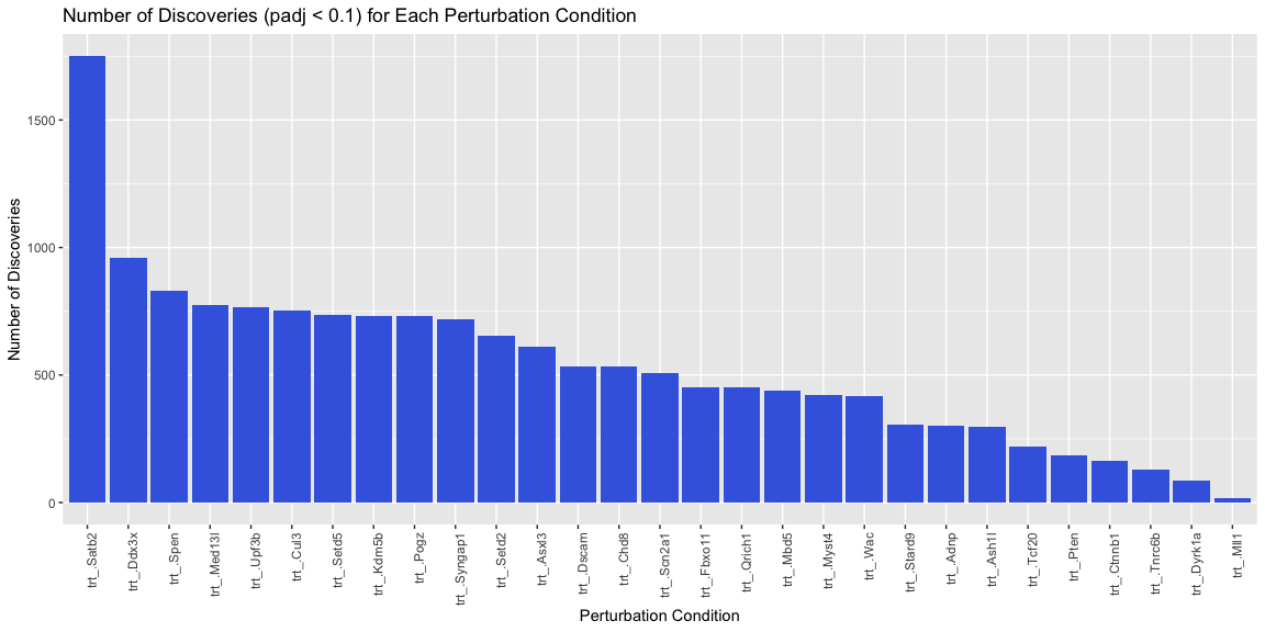
# Filter the results for significant discoveries
significant_discoveries <- df_res[df_res$padj < 0.1, ]

# Count the number of discoveries for each perturbation condition
discovery_counts <- as.data.frame(table(significant_discoveries$trt))
colnames(discovery_counts) <- c('Perturbation', 'Count')

# Order the discovery_counts by Count in descending order
discovery_counts <- discovery_counts %>% arrange(desc(Count))

# Set the factor levels of Perturbation to ensure ggplot respects the order
discovery_counts$Perturbation <- factor(discovery_counts$Perturbation, levels = discovery_counts$Perturbation)

# Plot the number of discoveries for each perturbation condition
ggplot(discovery_counts, aes(x = Perturbation, y = Count)) +
  geom_bar(stat = "identity", fill = "royalblue") +  theme(axis.text.x = element_text(angle = 90, hjust = 1)) +
  ggtitle('Number of Discoveries (padj < 0.1) for Each Perturbation Condition') +
  xlab('Perturbation Condition') +
  ylab('Number of Discoveries')